This post briefly summarizes our work on the Contrastive Perceptual Inference Network (CoPINet) for Raven’s Progressive Matrices (RPM). For further details, please refer to our NeurIPS 2019 paper.
1. Introduction
It was only until recently that the research community started to re-investigate tasks relying heavily on the ability of “thinking in pictures” with modern AI approaches, particularly spatial-temporal inductive reasoning; this line of work primarily focuses on Raven’s Progressive Matrices (RPM) [1]. In such a test, subjects are provided with two rows of figures following certain unknown rules and asked to pick the correct answer from the choices that would best complete the third row with a missing entry (see Figure 1(a) for an example). As shown in early works [2], despite the fact that visual elements are relatively straightforward, there is still a notable performance gap between human and machine visual reasoning in this challenging task.
We hypothesize that one missing ingredient that may result in this performance gap is a proper form of contrasting mechanism. Originated from perceptual learning, it is well established in the field of psychology and education that teaching new concepts by comparing with noisy examples is quite effective. We argue that such a contrast effect is essential to machines’ reasoning ability as well. In this work, we try to address a direct and challenging question: how to incorporate an explicit contrasting mechanism during model training in order to improve machines’ reasoning ability? Specifically, we come up with two levels of contrast in our model: a novel contrast module and a new contrast loss. At the model level, we design a permutation-invariant contrast module that summarizes the common features and distinguishes each candidate by projecting it onto its residual on the common feature space. At the objective level, we leverage ideas in contrastive estimation and propose a variant of Noise-Contrastive Estimation (NCE) loss.
Another reason why RPM is challenging for existing machine reasoning systems could be attributed to the demanding nature of the interplay between perception and inference. We propose to bridge this gap with a simple inference module jointly trained with the perception backbone; specifically, the inference module reasons about which category the current problem instance falls into. Instead of training the inference module to predict the ground-truth category, we borrow the basis learning idea and jointly learn the inference subsystem with perception.
In summary, this work makes four major contributions:
- We introduce two levels of contrast to improve machines’ reasoning ability in RPM. At the model level, we design a contrast module that aggregates common features and projects each candidate to its residual. At the objective level, we use an NCE loss variant instead of the cross-entropy to encourage contrast effects.
- We incorporate an inference module to learn with the perception backbone jointly. Instead of using ground-truth, we regularize it with a fixed number of bases.
- We make our model permutation-invariant in terms of swapped rows or columns and shuffled answer candidates, shifting the previous view of RPM from classification to ranking.
- Combining ideas above, we propose CoPINet that sets new state-of-the-art on two major datasets.
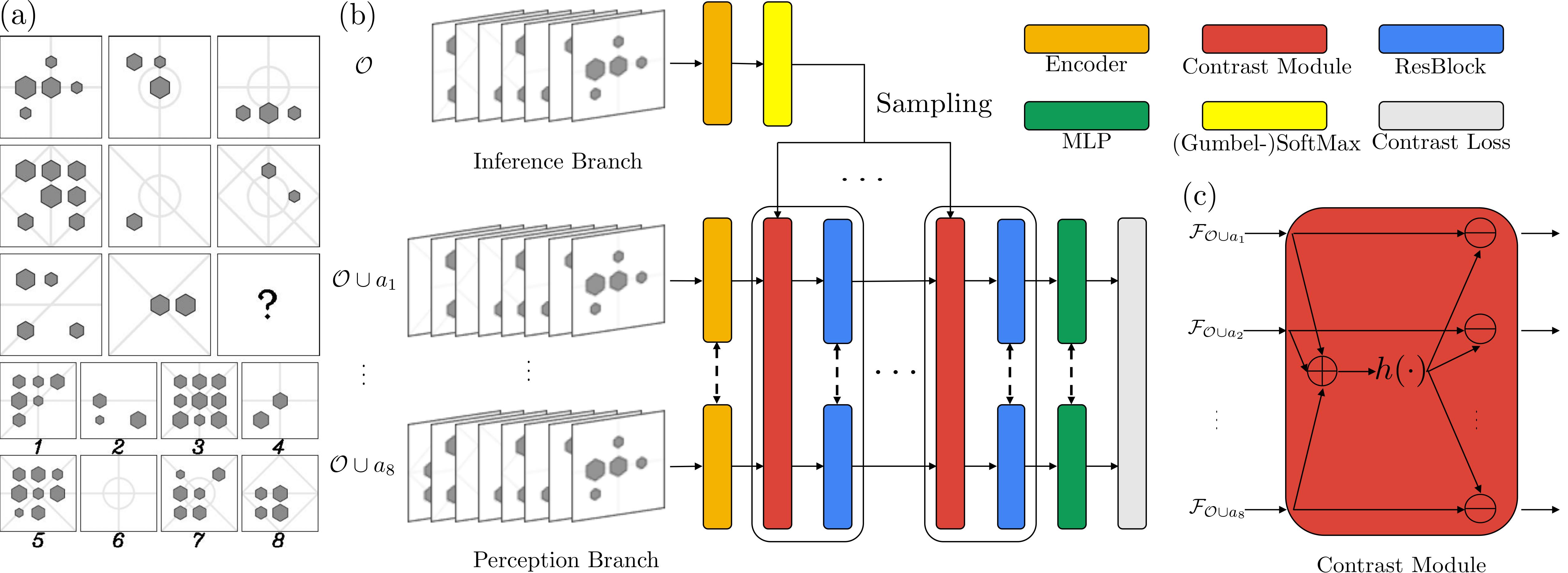 Figure 1. (a) An example of RPM. The hidden rule(s) in this problem can be denoted as \(\{[\text{OR}, \text{line}, \text{type}]\}\), where an OR operation is applied to the type attribute of all lines. It is further noted that the OR operation is applied row-wise, and there is only one choice that satisfies the row-wise OR constraint. Hence the correct answer should be \(5\). (b) The proposed CoPINet architecture. Given an RPM problem, the inference branch samples a most likely rule for each attribute based only on the context \(\mathcal{O}\) of the problem. Sampled rules are transformed and fed into each contrast module in the perception branch. Note that the combination of the contrast module and the residual block can be repeated. Dashed lines indicate that parameters are shared among the modules. (c) A sketch of the contrast module.
2. The CoPINet
The task of RPM can be formally defined as: given a list of observed images \(\mathcal{O} = \{o_i\}_{i = 1}^8\), forming a \(3\times3\) matrix with a final missing element, a solver aims to find an answer \(a_\star\) from an unordered set of choices \(\mathcal{A} = \{a_i\}_{i = 1}^8\) to best complete the matrix. Permutation invariance is a unique property for RPM problems: (1) The same set of rules is applied either row-wise or column-wise. Therefore, swapping the first two rows or columns should not affect how one solves the problem. (2) In any multi-choice task, changing the order of answer candidates should not affect how one solves the problem either. These properties require us to use a permutation-invariant encoder and reformulate the problem from a typical classification problem into a ranking problem. Formally, in a probabilistic formulation, we seek to find a model such that
\begin{equation} p(a_\star \vert \mathcal{O}) \geq p(a^\prime \vert \mathcal{O}), \quad \forall a^\prime \in \mathcal{A}, a^\prime \neq a_\star, \label{eqn:1} \tag{1} \end{equation}
where the probability is invariant when rows or columns in \(\mathcal{O}\) are swapped. This formulation also calls for a model that produces a density estimation for each choice, regardless of its order in \(\mathcal{A}\). To that end, we model the probability with a neural network equipped with a permutation-invariant encoder for each observation-candidate pair \(f(\mathcal{O} \cup a)\). However, we argue such a purely perceptive system is far from sufficient without contrasting and perceptual inference.
2.1 Contrasting
To provide the reasoning system with a mechanism of contrasting, we propose to explicitly build two levels of contrast: model-level contrast and objective-level contrast.
2.1.1 Model-level Contrast
As the central notion of contrast is comparing cases, we propose an explicit model-level contrasting mechanism in the following form,
\[\text{Contrast}(\mathcal{F}_{\mathcal{O} \cup a}) = \mathcal{F}_{\mathcal{O} \cup a} - h\left(\sum_{a^\prime \in \mathcal{A}}\mathcal{F}_{\mathcal{O} \cup a^\prime}\right)\]where \(\mathcal{F}\) denotes features of a specific combination and \(h(\cdot)\) summarizes the common features in all candidate answers. In our experiments, \(h(\cdot)\) is a composition of BatchNorm and Conv.
In a generalized setting, each \(\mathcal{O} \cup a\) could be abstracted out as an object. Then the design becomes a general contrast module, where each object is distinguished by comparing with the common features extracted from an object set.
We further note that the contrasting computation can be encapsulated into a single neural module and repeated: the addition and transformation are shared and the subtraction is performed on each individual element. See Figure 1(c) for a sketch of the contrast module. After such operations, permutation invariance of a model will not be broken.
2.1.2 Objective-level Contrast
To further enforce the contrast effects, we propose to use an NCE variant rather than the cross-entropy loss. We model the probability as:
\[p(a \vert \mathcal{O}) = \frac{1}{Z} \exp(f(\mathcal{O} \cup a)),\]where \(Z\) is the partition function, and our model \(f(\cdot)\) corresponds to the negative potential function.
We can take the log of both sides of Equation \(\ref{eqn:1}\) and rearrange terms:
\begin{equation} \log p(a_\star \vert \mathcal{O}) - \log p(a^\prime \vert \mathcal{O}) = f(\mathcal{O} \cup a_\star) - f(\mathcal{O} \cup a^\prime) \geq 0, \quad \forall a^\prime \in \mathcal{A}, a^\prime \neq a_\star. \end{equation}
This formulation could potentially lead to a max margin loss. However, we notice in our preliminary experiments that max margin is not sufficient; we realize it is inferior to make the negative potential of the wrong choices only slightly lower. Instead, we would like to further push the difference to infinity. To do that, we leverage the sigmoid function \(\sigma(\cdot)\) and train the model, such that:
\begin{equation} f(\mathcal{O} \cup a_\star) - f(\mathcal{O} \cup a^\prime) \rightarrow \infty \iff \sigma(f(\mathcal{O} \cup a_\star) - f(\mathcal{O} \cup a^\prime)) \rightarrow 1, \forall a^\prime \in \mathcal{A}, a^\prime \neq a_\star. \label{eqn:2} \tag{2} \end{equation}
However, we notice that the relative difference of negative potential is still problematic. We hypothesize this deficiency is due to the lack of a baseline—without such a regularization, the negative potential of wrong choices could still be very high, resulting in difficulties in learning the negative potential of the correct answer. To this end, we modify Equation \(\ref{eqn:2}\) into its sufficient conditions:
\begin{align} f(\mathcal{O} \cup a_\star) - b(\mathcal{O} \cup a_\star) \rightarrow \infty & \iff \sigma(f(\mathcal{O} \cup a_\star) - b(\mathcal{O} \cup a_\star)) \rightarrow 1 \newline f(\mathcal{O} \cup a^\prime) - b(\mathcal{O} \cup a^\prime) \rightarrow -\infty & \iff \sigma(f(\mathcal{O} \cup a^\prime) - b(\mathcal{O} \cup a^\prime)) \rightarrow 0, \end{align}
where \(b(\cdot)\) is a fixed baseline function and \(a^\prime \in \mathcal{A}, a^\prime \neq a_\star\). For implementation, \(b(\cdot)\) could be either a randomly initialized network or a constant. Since the two settings do not produce significantly different results in our preliminary experiments, we set \(b(\cdot)\) to be a constant to reduce computation.
We then optimize the network to maximize the following objective: \begin{equation} \ell = \log (\sigma(f(\mathcal{O} \cup a_\star) - b(\mathcal{O} \cup a_\star))) + \sum_{a^\prime \in \mathcal{A}, a^\prime \neq a_\star} \log (1 - \sigma(f(\mathcal{O} \cup a^\prime) - b(\mathcal{O} \cup a^\prime))) \label{eqn:loss}. \end{equation}
2.2 Perceptual Inference
A mere perceptive model for RPM is arguably not enough. Therefore, we propose to incorporate a simple inference subsystem into the model: the inference branch should be responsible for inferring the hidden rules in the problem. Specifically, we assume there are at most \(N\) attributes in each problem, each of which is subject to the governance of one of \(M\) rules. Then hidden rules \(\mathcal{T}\) in one problem instance can be decomposed into
\begin{equation} p(\mathcal{T} \vert \mathcal{O}) = \prod_{i = 1}^{N} p(t_{i} \vert \mathcal{O}), \end{equation}
where \(t_{i} = 1 \ldots M\) denotes the rule type on attribute \(n_i\). For the actual form of the probability of rules on each attribute, we propose to model it using a multinomial distribution.
If we treat rules as hidden variables, the log probability can be decomposed into
\begin{equation} \log p(a \vert \mathcal{O}) = \log \sum_{\mathcal{T}} p(a \vert \mathcal{T}, \mathcal{O}) p(\mathcal{T} \vert \mathcal{O}) = \log \mathbb{E}_{\mathcal{T} \sim p(\mathcal{T} \vert \mathcal{O})} [p(a \vert \mathcal{T}, \mathcal{O})]. \label{eqn:approx} \end{equation}
Note that writing the summation in the form of expectation affords sampling algorithms, which can be done on each individual attribute due to the independence assumption.
In addition, if we model \(p(\mathcal{T} \vert \mathcal{O})\) as an inference branch \(g(\cdot)\) and sample only once from it, the model can be modified into \(f(\mathcal{O} \cup a, \hat{\mathcal{T}})\) with \(\hat{\mathcal{T}}\) sampled from \(g(\mathcal{O})\). Following the same derivation above, we now optimize the new objective: \begin{equation} \ell = \log (\sigma(f(\mathcal{O} \cup a_\star, \hat{\mathcal{T}}) - b(\mathcal{O} \cup a_\star))) + \sum_{a^\prime \in \mathcal{A}, a^\prime \neq a_\star} \log (1 - \sigma(f(\mathcal{O} \cup a^\prime, \hat{\mathcal{T}}) - b(\mathcal{O} \cup a^\prime))). \label{eqn:final_loss} \end{equation} To sample from a multinomial, we could either use hard sampling like Gumbel-SoftMax or a soft one by taking expectation. We do not observe significant difference between the two settings.
The entire model is shown in Figure 1(b).
3. Experimental Results
We verify the effectiveness of our models on two major RPM datasets: RAVEN [2] and PGM [3]. Across all experiments, we train models on the training set, tune hyper-parameters on the validation set, and report the final results on the test set. All of the models are implemented in PyTorch and optimized using ADAM. While a good performance of WReN and ResNet+DRT relies on external supervision, such as rule specifications and structural annotations, the proposed model achieves better performance with only \(\mathcal{O}\), \(\mathcal{A}\), and \(a_\star\). Models are trained on servers with four Nvidia RTX Titans. For the WReN model, we use a public implementation that reproduces results. During training, we perform early-stop based on validation loss. We use the same network architecture and hyper-parameters in both RAVEN and PGM experiments. WReN-NoTag is a permutation-invariant version of WReN.
Table 1 shows the performance of different models on the RAVEN dataset. The first part shows the general performance while the second shows the ablation study. As shown, CoPINet achieves the best performance among existing methods and the contrast module, the contrast loss, and the perceptual inference, all help the model improve performance, with the contrast module most significantly. For detailed analysis, please refer to our paper.
| Method | Acc | Center | 2x2Grid | 3x3Grid | L-R | U-D | O-IC | O-IG |
|---|---|---|---|---|---|---|---|---|
| LSTM | 13.07% | 13.19% | 14.13% | 13.69% | 12.84% | 12.35% | 12.15% | 12.99% |
| WReN-NoTag-Aux | 17.62% | 17.66% | 29.02% | 34.67% | 7.69% | 7.89% | 12.30% | 13.94% |
| CNN | 36.97% | 33.58% | 30.30% | 33.53% | 39.43% | 41.26% | 43.20% | 37.54% |
| ResNet | 53.43% | 52.82% | 41.86% | 44.29% | 58.77% | 60.16% | 63.19% | 53.12% |
| ResNet+DRT | 59.56% | 58.08% | 46.53% | 50.40% | 65.82% | 67.11% | 69.09% | 60.11% |
| CoPINet | 91.42% | 95.05% | 77.45% | 78.85% | 99.10% | 99.65% | 98.50% | 91.35% |
| WReN-NoTag-NoAux | 15.07% | 12.30% | 28.62% | 29.22% | 7.20% | 6.55% | 8.33% | 13.10% |
| WReN-Tag-NoAux | 17.94% | 15.38% | 29.81% | 32.94% | 11.06% | 10.96% | 11.06% | 14.54% |
| WReN-Tag-Aux | 33.97% | 58.38% | 38.89% | 37.70% | 21.58% | 19.74% | 38.84% | 22.57% |
| CoPINet-Backbone-XE | 20.75% | 24.00% | 23.25% | 23.05% | 15.00% | 13.90% | 21.25% | 24.80% |
| CoPINet-Contrast-XE | 86.16% | 87.25% | 71.05% | 74.45% | 97.25% | 97.05% | 93.20% | 82.90% |
| CoPINet-Contrast-CL | 90.04% | 94.30% | 74.00% | 76.85% | 99.05% | 99.35% | 98.00% | 88.70% |
| Human | 84.41% | 95.45% | 81.82% | 79.55% | 86.36% | 81.81% | 86.36% | 81.81% |
| Solver | 100% | 100% | 100% | 100% | 100% | 100% | 100% | 100% |
Table 1. Testing accuracy of models on RAVEN. Acc denotes the mean accuracy of each model. L-R denotes the Left-Right configuration, U-D Up-Down, O-IC Out-InCenter, and O-IG Out-InGrid.
Table 2 shows the performance of existing methods on the PGM dataset. Among all permutation-invariant methods, CoPINet again achieves the best performance. The ablation study on Table 3 also leads to the conclusions drawn from RAVEN.
| Method | CNN | LSTM | ResNet | Wild-ResNet | WReN-NoTag-Aux | CoPINet |
|---|---|---|---|---|---|---|
| Acc | 33.00% | 35.80% | 42.00% | 48.00% | 49.10% | 56.37% |
Table 2. Testing accuracy of models on PGM. Acc denotes the mean accuracy of each model.
| Method | WReN-NoTag-NoAux | WReN-NoTag-Aux | WReN-Tag-NoAux | WReN-Tag-Aux |
|---|---|---|---|---|
| Acc | 39.25% | 49.10% | 62.45% | 77.94% |
| Method | CoPINet-Backbone-XE | CoPINet-Contrast-XE | CoPINet-Contrast-CL | CoPINet |
| Acc | 42.10% | 51.04% | 54.19% | 56.37% |
Table 3. Ablation study on PGM.
4. Conclusion
In this work, we aim to improve machines’ reasoning ability in “thinking in pictures” by jointly learning perception and inference via contrasting. Specifically, we introduce the contrast module, the contrast loss, and the joint system of perceptual inference. We also require our model to be permutation-invariant. In a typical and challenging task of this kind, Raven’s Progressive Matrices (RPM), we demonstrate that our proposed model—Contrastive Perceptual Inference network (CoPINet)—achieves the new state-of-the-art for permutation-invariant models on two major RPM datasets. Further ablation studies show that all the three proposed components are effective towards improving the final results, especially the contrast module. It also shows that the permutation invariance forces the model to understand the effects of different choices on the compatibility of an entire RPM matrix, rather than remembering the positional association and shortcutting the solutions.
Performance, however, is definitely not the end goal in the line of research on relational and analogical visual reasoning: other dimensions for measurements include generalization, generability, and transferability. Is it possible for a model to be trained on a single configuration and generalize to other settings? Can we generate the final answer based on the given context panels, in a similar way to the top-down and bottom-up method jointly applied by humans for reasoning? Can we transfer the relational and geometric knowledge required in the reasoning task from other tasks? Questions like these are far from being answered and we hope this work would inspire future work into these problems.
If you find the paper helpful, please cite us.
@inproceedings{zhang2019learning,
    title={Learning perceptual inference by contrasting},
    author={Zhang, Chi and Jia, Baoxiong and Gao, Feng and Zhu, Yixin and Lu, Hongjing and Zhu, Song-Chun},
    booktitle={Advances in Neural Information Processing Systems},
    year={2019}
}
References
[1] Raven, John Carlyle. Raven’s progressive matrices and vocabulary scales. Oxford pyschologists Press, 1998.
[2] Zhang, Chi, et al. “Raven: A dataset for relational and analogical visual reasoning.” Proceedings of the IEEE Conference on Computer Vision and Pattern Recognition. 2019.
[3] Santoro, Adam, et al. “Measuring abstract reasoning in neural networks.” International Conference on Machine Learning. 2018.
-
Previous
RAVEN: A Dataset for Relational and Analogical Visual rEasoNing -
Next
Abstract Spatial-Temporal Reasoning via Probabilistic Abduction and Execution